Purpose of statistical programming software

Unlike spreadsheet applications (like Excel) or point-and-click statistical analysis software (SPSS), statistical programming software is based around a script-file where the user writes a series of commands to be performed,

Advantages of statistical programming software

• Data analysis process is reproducible and transparent.

• Due to the open-ended nature of language-based programming, there is far more versatility and customizability in what you can do with data.

• Typically statistical programming software has a much more comprehensive range of built-in analysis functions than spreadsheets etc.

Characteristics of R

• R is an open-source language specifically designed for statistical computing (and it’s the most popular choice among statisticians)

• Because of its popularity and open-source nature, the R community’s package development means it has the most prewritten functionality of any data analysis software.

• Differs from software like Stata, however, in that while you can use prewritten functions, it is equally adept at programming solutions for yourself.

• Because it’s usage is broader, R also has a steeper learning curve than Stata.

Comparison to other statistical programming software

• Stata: The traditional choice of (academic) economists.
  • Stata is more specifically econometrics focused and is much more command-oriented. Easier to use for standard applications, but if there’s not a Stata command for what you want to do, it’s harder to write something yourself.
    
  • Stata is also very different than R in that you can only ever work with one dataset at a time, while in R, it’s typical to have a number of data objects in the environment.

• SAS: Similar to Stata, but more commonly used in business & the private sector, in part because it’s typically more convenient for massive datasets. Otherwise, I think it’s seen as a bit older and less user-friendly.

• Python: Another option based more on programming from scratch and with less prewritten commands. Python isn’t specific to math & statistics, but instead is a general programming language used across a range of fields.
  Probably the most similar software choice to R at this point, with better general use (and programming ease) at the cost of less package development specific to econometrics/data analysis.

• Matlab: Popular in macroeconomics and theory work, not so much in empirical work. Matlab is powerful, but is much more based on programming “from scratch” using matrices and mathematical expressions.

Useful resources for learning R

• DataCamp: interactive online lessons in R.
  • Some of the courses are free (particularly community-written lessons like the one you’ll do today), but for paid courses, DataCamp costs about 300 SEK / mo.

• RStudio Cheat Sheets: Very helpful 1-2 page overviews of common tasks and packages in R.

• Quick-R: Website with short example-driven overviews of R functionality.

• StackOverflow: Part of the Stack Exchange network, StackOverflow is a Q&A community website for people who work in programming. Tons of incredibly good R users and developers interact on StackExchange, so it’s a great place to search for answers to your questions.

• R-Bloggers: Blog aggregagator for posts about R. Great place to learn really cool things you can do in R.

• R for Data Science: Online version of the book by Hadley Wickham, who has written many of the best packages for R, including the Tidyverse, which we will cover.

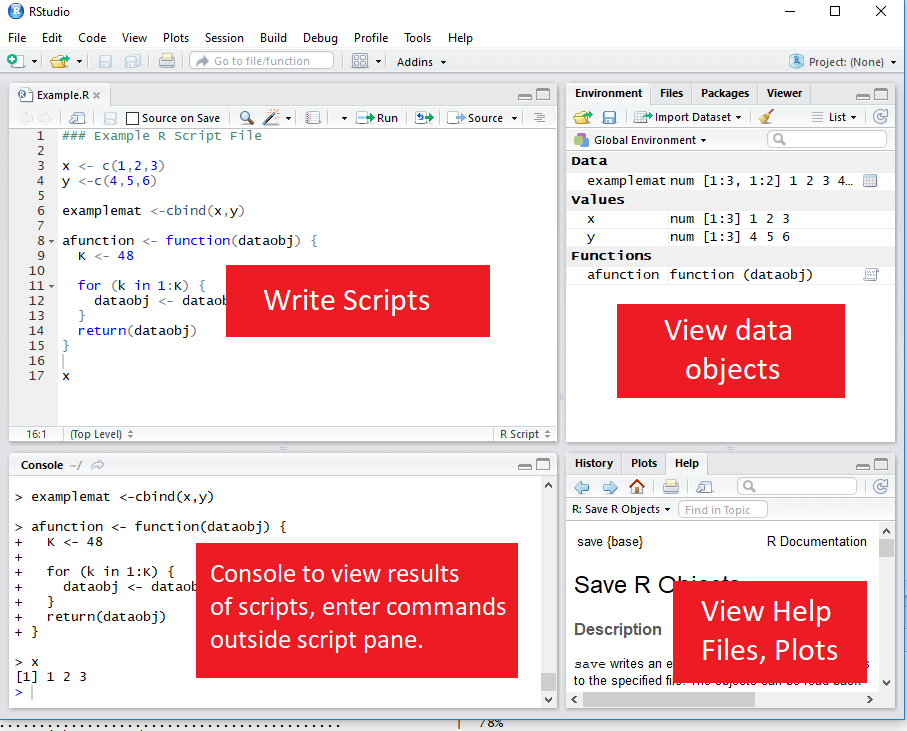
RStudio GUI

RStudio is an is an integrated development environment (IDE).

This means that in addition to a script editor, it also let’s you view your environments, data objects, plots, help files, etc directly within the application.

Executing code from the script

To execute a section of code, highlight the code and click “Run” or use Ctrl-Enter.

• For a single line of code, you don’t need to highlight, just click into that line.

• To execute the whole document, the hotkey is Ctrl-Shift-Enter.

Style advise

Unlike Stata, with R you don’t need any special code to write multiline code - it’s already the default (functions are written with parentheses, so its clear when the line actually ends.)

• So there’s no excuse for really long lines. Accepted style suggests using a 80-character limit for your lines.

• RStudio has the option to show a guideline for margins. Use it!
  • Go to Tools -> Global Options -> Code -> Display, then select Show Margin and enter 80 characters.

You can also write multiple expressions on the same line by using ; as a manual line break.

Comments

To create a comment in R, use a hash ( #. For example:

# Here I add 2 + 2
2 + 2

## [1] 4

Help files in R

You can access the help file for any given function using the help function. You can call it a few different ways:

1. In the console, use help()
2. In the console, use ? immediately followed by the name of the function (no space inbetween)
3. In the Help pane, search for the function in question.

? is shorter, so that’s the most frequent method.

# Help on the lm (linear regression) function
?lm

Setting the working directory

To set the working directory, use the function setwd(). The argument for the function is simply the path to the working directory, in quotes.

However: be sure that the slashes in the path are forward slashes (/). For Windows, this is not the case if you copy the path from File Explorer so you’ll need to change them.

# Set Working Directory
setwd("C:/Users/Andrew/Documents/MyProject")

Math operations in R

Examples of basic mathematical operations in R:

# Addition and Subtraction
2 + 2

## [1] 4

# Multiplication and Division
2*2 + 2/2

## [1] 5

# Exponentiation and Logarithms
2^2 + log(2)

## [1] 4.693147

Logical operations in R

You can also evaluate logical expressions in R

## Less than
5 <= 6

## [1] TRUE

## Greater than or equal to
5 >= 6

## [1] FALSE

## Equality
5 == 6

## [1] FALSE

## Negatiion
5 != 6

## [1] TRUE

You can also use AND ( &) and OR ( |) operation with logical expressions:

## Is 5 equal to 5 OR 5 is equal to 6
(5 == 5) | (5 == 6)

## [1] TRUE

## 5 less 6 AND 6 < 5
(5 < 6) & (7 < 6)

## [1] FALSE

Defining an object

To define an object, use <-. For example

# Assign 2 + 2 to the variable x
x <- 2 + 2

Note: In R, there is no distinction between defining and redefining an object (a la gen/replace in Stata).

y <- 4 # Define y
y <- y^2 # Redefine y
y #Print y 

## [1] 16

Data classes

Data elements in R are categorized into a few seperate classes (ie types)

• numeric: Data that should be interpreted as a number.

• logical: Data that should be interpreted as a logical statment, ie. TRUE or FALSE.

• character: Strings/text.
  • Note, depending on how you format your data, elements that may look like logical or numeric may instead be character.

• factor: In affect, a categorical variable. Value may be text, but R interprets the variable as taking on one of limited number of possible values (e.g. sex, municipality, industry etc)

What’s the object class?

a <- 2; class(a)

## [1] "numeric"

b <- "2"; class(b)

## [1] "character"

c <- TRUE; class(c)

## [1] "logical"

d <- "True"; class(d)

## [1] "character"

Vectors

The basic data structure containing multiple elements in R is the vector.

• An R vector is much like the typical view of a vector in mathematics, ie it’s basically a 1D array of elements.

• Typical vectors are of a single-type (these are called atomic vectors).

• A list vector can also have elements of different types.

Creating vectors

To create a vector, use the function c().

# Create `days` vectors
days <- c("Mon","Tues","Wed",
           "Thurs", "Fri")

# Create `temps` vectors
temps <- c(13,18,17,20,21)
# Display `temps` vector
temps

## [1] 13 18 17 20 21

Naming vectors

You can name a vector by assigning a vector of names to c(), where the vector to be named goes in the parentheses.

# Assign `days` as names for `temps` vector
names(temps) <- days 
# Display `temps` vector
temps

##   Mon  Tues   Wed Thurs   Fri 
##    13    18    17    20    21

Subsetting vectors

There are multiple ways of subsetting data in R. One of the easiest methods for vectors is to put the subset condition in brackets:

# Subset temps greater than or equal to 10
temps[temps>=18]

##  Tues Thurs   Fri 
##    18    20    21

Operations on vectors

Operations on vectors are element-wise. So if 2 vectors are added together, each element of the \(2^{nd}\) vector would be added to the corresponding element from the \(1^{st}\) vector.

# Temp vector for week 2
temps2 <- c(8,10,10,15,16)
names(temps2) <- days
# Create average temperature by day
avg_temp <- (temps + temps2) / 2
# Display `avg_temp`
avg_temp

##   Mon  Tues   Wed Thurs   Fri 
##  10.5  14.0  13.5  17.5  18.5

Matrices

• Data in a 2-dimensional structure can be represented in two formats, as a matrix or as a data frame.

• A matrix is used for 2D data structures of a single data type (like atomic vectors).
  • Usually, matrices are composed of numeric objects.

• To create a matrix, use the matrix() command.

The syntax of ** matrix() ** is:

matrix(x, nrow=a, ncol=b, byrow=FALSE/TRUE)

-x is the data that will populate the matrix.

-nrow and ncol specify the number of rows and columns, respectively.
Generally need to specify just 1 since the number of elements and a single condition will determine the other.

-byrow specifies whether to fill in the elements by row or column. The default is byrow=FALSE, ie the data is filled in by column.

Creating a matrix from scratch

A simple example of creating a matrix would be:

matrix(1:6, nrow=2, ncol=3, byrow=FALSE)

##      [,1] [,2] [,3]
## [1,]    1    3    5
## [2,]    2    4    6

Note the difference in appearance if we instead byrow=TRUE

matrix(1:6, nrow=2, ncol=3, byrow=TRUE)

##      [,1] [,2] [,3]
## [1,]    1    2    3
## [2,]    4    5    6

Using the same c() function as in the creation of a vector, we can specify the values of a matrix:

matrix(c(13,18,17,20,21,
         8,10,10,15,16), 
         nrow=2, byrow=TRUE)

##      [,1] [,2] [,3] [,4] [,5]
## [1,]   13   18   17   20   21
## [2,]    8   10   10   15   16

• Note that the line breaks in the code are purely for
  readability purposes. Unlike Stata, R allows you to break
  code over multiple lines without any extra line break syntax.

Creating a matrix from vectors

Instead of entering in the matrix data yourself, you may want to make a matrix from existing data vectors:

# Create temps matrix
temps.matrix <- matrix(c(temps,temps2), nrow=2, 
                        ncol=5, byrow=TRUE)
# Display matrix
temps.matrix

##      [,1] [,2] [,3] [,4] [,5]
## [1,]   13   18   17   20   21
## [2,]    8   10   10   15   16

Naming rows and columns

-Naming rows and columns of a matrix is pretty similar to naming vectors.

-Only here, instead of using names(), we use rownames() and colnames()

# Create temps matrix
rownames(temps.matrix) <- c("Week1", "week2")
colnames(temps.matrix) <- days
# Display matrix
temps.matrix

##       Mon Tues Wed Thurs Fri
## Week1  13   18  17    20  21
## week2   8   10  10    15  16

Matrix operations

In R, matrix multiplication is denoted by %\(*\)%, as in A %\(*\)% B

A * B instead performs element-wise (Hadamard) multiplication of matrices, so that A * B has the entries \(a_1 b_1\), \(a_2 b_2\) etc.

• An important thing to be aware of with R’s A * B notation, however, is that if either of the terms is a 2D vector, the terms of this vector will be distributed elementwise to each colomn of the matrix.

Elementwise operations with a vector and Matrix

vecA; matB

## [1] 1 2

##      [,1] [,2] [,3]
## [1,]    1    2    3
## [2,]    4    5    6

vecA * matB

##      [,1] [,2] [,3]
## [1,]    1    2    3
## [2,]    8   10   12

Creating a data frame

• Most of the time you’ll probably be working with datasets that are recognized as data frames when imported into R.

• But you can also easily create your own data frames.

• This might be as simple as converting a matrix to a data frame:

mydf <- as.data.frame(matB)
mydf

##   V1 V2 V3
## 1  1  2  3
## 2  4  5  6

• Another way of creating a data frame is to combine other vectors or matrices (of the same length) together.

mydf <- data.frame(vecA,matB)
mydf

##   vecA X1 X2 X3
## 1    1  1  2  3
## 2    2  4  5  6

Defining a column of a data frame (or other 2D object):

Once you have a multidimensional data object, you will usually want to create or manipulate particular columns of the object.

The default way of invoking a named column in R is by appending a dollar sign and the column name to the data object.

wages # View wages data frame

##        wage schooling    sex exper
## 1 134.23058        13 female     8
## 2 249.67744        13 female    11
## 3  53.56478        10 female    11

wages$expersq <- wages$exper^2; wages  # Add expersq

##        wage schooling    sex exper expersq
## 1 134.23058        13 female     8      64
## 2 249.67744        13 female    11     121
## 3  53.56478        10 female    11     121

Viewing the structure of a data frame

Like viewing the class of a homogenous data object, it’s often helpful to view the structure of data frames (or other 2D objects).

• You can easily do this using the ** str() ** function.

# View the structure of the wages data frame
str(wages)

## 'data.frame':    3 obs. of  5 variables:
##  $ wage     : num  134.2 249.7 53.6
##  $ schooling: int  13 13 10
##  $ sex      : Factor w/ 2 levels "female","male": 1 1 1
##  $ exper    : int  8 11 11
##  $ expersq  : num  64 121 121

Changing the structure of a data frame

A common task is to redefine the classes of columns in a data frame.

• Common commands can help you with this when the data is formatted suitably:

  • as.numeric() will take data that looks like numbers but are formatted as characters/factors and change their formatting to numeric.

  • as.character() will take data formatted as numbers/factors and change their class to character.

  • as.factor() will reformat data as factors, taking by default the unique values of each column as the possible factor levels.

More about factors

Although as.factor() will suggest factors from the data, you may want more control over how factors are specified.

With the factor() function, you supply the possible values of the factor and you can also specify ordering of factor values if your data is ordinal.

str(affairs) # view structure

## 'data.frame':    3 obs. of  4 variables:
##  $ affairs: num  0 0 1
##  $ yrsmarr: num  15 1.5 7
##  $ child  : Factor w/ 2 levels "no","yes": 2 1 2
##  $ mrating: int  1 5 3

## Format mrating as ordered factor
affairs$mrating <-factor(affairs$mrating, 
   levels=c(1,2,3,4,5), ordered=TRUE)
str(affairs)

## 'data.frame':    3 obs. of  4 variables:
##  $ affairs: num  0 0 1
##  $ yrsmarr: num  15 1.5 7
##  $ child  : Factor w/ 2 levels "no","yes": 2 1 2
##  $ mrating: Ord.factor w/ 5 levels "1"<"2"<"3"<"4"<..: 1 5 3

Selections and subsets in data frames

Similar to subsetting a vector, matrices & data frames can also be subsetted for both rows and columns by placing the selection arguments in brackets after the name of the data object:

Arguments can be:

• Row or column numbers (eg mydf[1,3])

• Row or column names

• Rows (ie observations) that meet a given condition

# Subset of wages df with schooling > 10, exper > 10
wages[(wages$schooling > 10) & (wages$exper > 10),]

##       wage schooling    sex exper expersq
## 2 249.6774        13 female    11     121