Revisiting basics

Assignment Operator

So far, when changing a data object, we have always been a bit repetitive:

mydataframe <-  mydataframe %>% rename(NewVarName = OldVarName)

Along with the standard pipe (%>%), by loading the magrittr package, you can also use the so-called “assignment pipe” (%<>%).

The above rename with the assignment pipe appears as:

mydataframe %<>% rename(NewVarName = OldVarName)

Lists

Another subtlety glossed over so far are lists.

As mentioned in module 1, vectors come in two forms: atomic vectors (with a single data type) and lists (with heterogenous data types).
Lists can take as inputs not only single-valued elements, but also vectors or data frames.
Creating a list from other objects is done with the list() function. The syntax of list is:

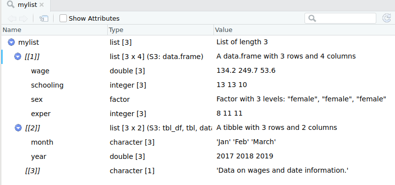
List Creation Example

wages_df; date_df; description

##        wage schooling    sex exper
## 1 134.23058        13 female     8
## 2 249.67744        13 female    11
## 3  53.56478        10 female    11

##   month year
## 1   Jan 2017
## 2   Feb 2018
## 3 March 2019

## [1] "Data on wages and date information."

mylist <- list(wages = wages_df, dates = date_df, description)

Where wages_df and date_df are data frames and description is a single character element.

List Creation Example ctd

Subsetting a list

To subset a vector/matrix/data frame, one uses single brackets, eg mydf[,].
To refer to an object of a list, use double brackets.

mylist[[3]]

## [1] "Data on wages and date information."

Note: The function list() does not take transfer the names of the data frames, so you will need to either subset by position or assign names to the list objects.

Extracting a list

An easy way of extracting an object from a list is with the extract2() function from magrittr. This allows you to extra a given list object by name or position.

wage_data <- mylist %>% extract2(1)
wage_data

##        wage schooling    sex exper
## 1 134.23058        13 female     8
## 2 249.67744        13 female    11
## 3  53.56478        10 female    11

The unlist function

Instead of creating more complicated data objects, sometimes formatted as list into a simple (atomic) vector. The unlist() function does this.

Example:

simple_list <-list(1,2,3,4)
str(simple_list)

## List of 4
##  $ : num 1
##  $ : num 2
##  $ : num 3
##  $ : num 4

simple_list %<>% unlist() %>% str()

##  num [1:4] 1 2 3 4

Iteration

For loops

For tasks that you want to iterate over multiple data frames/variables/elements, you may want to think about creating a loop.

A loop performs a function/functions multiple times, across either a list of objects or a set of index values.

Syntax:

for(indexname in range) {
  do stuff
}

For loop across numeric values

for (i in 1:4){
  print(i^2)
}

## [1] 1
## [1] 4
## [1] 9
## [1] 16

For loop across named elements

You can also loop over elements instead of values.

In the last module exercises, you had to convert the type of many variables. Here’s one way you could do that with a loop:

nlsy97 <- import("./data/nlsy97.rds")
factor.vars <- c("personid","year","sex","race","region","schooltype")
  for (i in factor.vars){
   nlsy97[,i] %<>% unlist() %>% as.factor()
  }

The map() function

For iterations over vectors and dataframes, the map() function is a great alternative to the for loop.

Map functions take a user-supplied function and iterate it over:

Elements for a vector
Objects of a list
Columns of a data frame

Map functions are much simpler to write than loops and are also generally a good bit faster.

Sidenote: Map is a part of the tidyverse collection of packages. In base R, the apply() family of functions does roughly the same thing, but map() simplifies and improves this task.

Using the map() function

Syntax:

map(data, fxn, option1, option2...)

Example:

nlsy97[,factor.vars] %<>% map(as.factor)

Using class-specific map variants

There are multiple map variants that enforce a given data type on results. You should use these whenever you want output of a certain class.

map_lgl for logical vector
map_dbl for numeric vector
map_chr for character vector
map_df for a data frame

Example of difference with class-specific map variants

nlsy.sub <- nlsy97 %>% select(parentincome, motheredyrs, gpa)
nlsy.sub %>% map_dbl(IQR, na.rm=TRUE)

## parentincome  motheredyrs          gpa 
##   55947.2500       3.0000       2.8075

nlsy.sub %>% map(IQR, na.rm=TRUE)

## $parentincome
## [1] 55947.25
## 
## $motheredyrs
## [1] 3
## 
## $gpa
## [1] 2.8075

Using map() with anonymous functions

map() works with not only predefined functions, but also “anonymous functions”— unnamed functions defined inside of map().

Suppose I want the z-standardized values of the variables from the previous example:

# Create Z Transform
ztransform <- map_df(nlsy.sub, function(x) 
  (x - mean(x,  na.rm=TRUE)) / sd(x, na.rm=TRUE)
  )

### Did it work?

# Means
map_dbl(ztransform, function(x) 
  round(mean(x, na.rm=TRUE),10))

## parentincome  motheredyrs          gpa 
##            0            0            0

# Standard deviations
map_dbl(ztransform, function(x) 
  round(sd(x, na.rm=TRUE),10))

## parentincome  motheredyrs          gpa 
##            1            1            1

Conditional Statements

If statements

“If statements” are also a useful part of programming, either in conjunction with iteration or seperately.

An if statement performs operations only if a specified condition is met.
- An important thing to know, however, is that if statements evaluate conditions of length one (ie non-vector arguments).
- We will cover a vector equivalent to the if statement shortly.

Syntax

if(condition){
     do stuff
    }

Example of an if statement

In the for loop example, the loop was indexed over only the columns of indicator codes.
Equally, the loop could be done over all columns with an if-statement to change only the indicator codes.

for (j in colnames(nlsy97)){
  
  if(j %in% factor.vars){
      nlsy97[,j] %<>% unlist() %>% as.factor()
  }
}

Multiple conditions

You can encompass several conditions using the else if and catch-all else control statements.

if (condition1) {
do stuff
} else if (condition2) {
do other stuff
} else {
do other other stuff
}

Vectorized if statements

As alluded to earlier, if statements can’t test-and-do for vectors, but only single-valued objects.
Most of the time, you probably want to use conditional statements on vectors. The vector equivalent to the if statement is ifelse()

Syntax:

ifelse(condition, true_statement, false_statement)

The statements returned can be simple values, but they can also be functions or even further conditions. You can easily nest multiple ifelses if desired.

An ifelse example

 numbers <- sample(1:30, 7); numbers

## [1] 29 11 13 22 27 12 30

 ifelse(numbers %% 2 == 0,"even","odd")

## [1] "odd"  "odd"  "odd"  "even" "odd"  "even" "even"

Note: What if we tried a normal if statement instead?

 if(numbers %% 2 == 0){
   print("even")} else{
     print("odd")}

## [1] "odd"

Multiple vectorized if statements

A better alternative to multiple nested ifelse statements is the tidyverse case_when function.

Syntax:

case_when(
  condition1 ~ statement1,
  condition2 ~ statement2,
  condition3 ~ statement3,
)

A case_when example

nums_df <- numbers %>% as.tibble() %>% 
  mutate(interval = case_when(
  (numbers > 0 & numbers <= 10) ~ "1-10",
  (numbers > 10 & numbers <= 20) ~ "10-20",
  (numbers > 20 & numbers <= 30) ~ "20-30"))
nums_df[1:4,]

## # A tibble: 4 x 2
##   value interval
##   <int> <chr>   
## 1    29 20-30   
## 2    11 10-20   
## 3    13 10-20   
## 4    22 20-30

Functions

When you should write a function

If you find yourself performing the same specific steps more than a couple of times (perhaps with slight variations), then you should consider writing a function.

A function can serve essentially as a wrapper for a series of steps, where you define generalized inputs/arguments.

Writing a function

Ingredients:

Function name
Arguments
Function body

Syntax:

function_name <- function(arg1, arg2, ...){
  do stuff
}

Function example

Let’s turn the calculation of even or odd that was completed earlier into a function:

# Make odd function
odd <- function(obj){
   ifelse(obj %% 2 == 0,"even","odd")
}

Notice that obj here is a descriptive placeholder name for the data object to be supplied as an argument for the function.

odd(numbers)

## [1] "odd"  "odd"  "odd"  "even" "odd"  "even" "even"

RStudio’s “Extract Function”

A useful way of writing simple functions when you’ve already written the code for a specific instance is to use RStudio’s Extract Function option, which is available from the code menu.

Extract function will take the code chunk and treat any data objects referenced but not created within the chunk as function arguments.

Joins

Merging data

Shifting gears from programming…

Another staple task in applied work is combining data from multiple data sets. The tidyverse set of packages includes several useful types of merges (or “joins”):

left_join() Appends columns from dataset B to dataset A, keeping all observations in dataset A.
inner_join() Appends columns together, keeping only observations that appear in both dataset A and B.
semi_join() Keeps only columns of dataset A for observations that appear in both dataset A and B.
anti_join() Keeps only columns of dataset A for observations that do not appear in both dataset A and B.

Joining using keys

The starting point for any merge is to enumerate the column or columns that uniquely identify observations in the dataset.

For cross-sectional data, this might be a personal identifier or (for aggregate data) something like municipality, state, country, etc.
For panel data, this will typically be both the personal/group identifier and a timing variable, for example Sweden in 2015 in a cross-country analysis.

Mismatched key names across datasets

Sometimes the names of the key variables are different across datasets.

You could of course rename the key variables to be consistent.
But mismatched key names are easily handled by the tidyverse join functions.

Syntax:

join_function(x, y, by = c("x_name" = "y_name"))

left_join

The left_join() is the most frequent type of join, corresponding to a standard merge in Stata.

left_join simply appends additional variables from a second dataset to a main dataset, keeping all the observations (rows) of the first dataset.

Syntax:

left_join(x, y, by = "key")

If the key is muliple columns, use c() to list them.

left_join example

# Look at the datasets
earnings

##   person_id wage
## 1       001  150
## 2       002   90
## 3       003  270

educ

##   person_id schooling
## 1       001        12
## 2       003         8
## 3       004        16

# Combine data
combined_data <- left_join(earnings, educ, 
                           by="person_id")

# Print data
combined_data

##   person_id wage schooling
## 1       001  150        12
## 2       002   90        NA
## 3       003  270         8

Notice that schooling is equal to NA for person ‘002’ because that person does not appear in the educ dataset.

inner_join

If you want to combine the variables of two data sets, but only keep the observations present in both datasets, use the inner_join() function.

combined_data <- inner_join(earnings, educ, 
                            by="person_id")
combined_data

##   person_id wage schooling
## 1       001  150        12
## 2       003  270         8

semi_join

To keep using only the variables in the first dataset, but where observations in the first dataset are matched in the second dataset, use semi_join().

semi_join is an example of a filtering join. Filtering joins don’t add new columns, but instead just filter observations for matches in a second dataset.
left_join and inner_join are instead known as mutating joins, because new variables are added to the dataset.

filtered_data <- semi_join(earnings, educ, by="person_id")
filtered_data

##   person_id wage
## 1       001  150
## 2       003  270

anti_join

Another filtering join is anti_join(), which filters for observations that are not matched in a second dataset.

filtered_data <- anti_join(earnings, educ, 
                           by="person_id")
filtered_data

##   person_id wage
## 1       002   90

There are still other join types, which you can read about here.

Appending data

Finally, instead of joining different datasets for the same individuals, sometimes you want to join together files that are for different individuals within the same dataset.

When join data where the variables for each dataset are the same, but the observations are different, this is called appending data.

The function for appending data in the tidyverse is:

bind_rows(list(dataframe1,dataframe2,...))

Manipulating text

Concatenating strings

The last type of data preparation that we will cover in this course is manipulating string data.

The simplest string manipulation may be concatenating (ie combining) strings.
- A great function for combining string in R is the glue() function, part of the Tiydverse glue package.
The glue function lets you reference variable values inside of text strings by writing the variable in curly brackets {} inside of the string.

Glue Example

date_df %<>% mutate(
   say.month = glue("The month is {month}"),
   mo.yr = glue("{month} {year}")
 )
date_df

##   month year          say.month      mo.yr
## 1   Jan 2017   The month is Jan   Jan 2017
## 2   Feb 2018   The month is Feb   Feb 2018
## 3 March 2019 The month is March March 2019

Glue Example 2

numbers <- c(1,2,3)
for (i in numbers){
  print(glue("The magic number is {i}"))
}

## The magic number is 1
## The magic number is 2
## The magic number is 3

Extracting and replacing parts of a string

Other common string manipulating tasks include extracting or replacing parts of a string. These are accomplished via the str_extract() and str_replace() from the Tidyverse stringr package.

We saw examples of these two functions in the last seminar exercise:

The arguments for each function are:

str_extract(string_object, "pattern_to_match")
str_replace(string_object, "pattern_to_match","replacement_text")

By default, both function operate on the first match of the specified pattern. To operate on all matchs, add “_all" to the function name, as in:

str_extract_all(string_object, "pattern_to_match")

Extract and replace example

In the last seminar, we created a “year” column from years indicated in the “variable” column text via the expression:

nlsy97$year <- str_extract(nlsy97$variable, "[0-9]+")

After creating the “year” column, we then removed the year values from the values of the “variable” column by replacing these numbers with an empty string.

nlsy97$variable <- str_replace(nlsy97$variable, "[0-9]+","")

Trimming a string

When working with formatted text, a third common task is to remove extra spaces before or after the string text.

This is done with the str_trim() function. The syntax is:

str_trim(string, side = "left"/"right"/"both")

Note, when printing a string, any formatting characters are shown. To view how the string looks formatted, use the ViewLines() function.

Using regular expressions with strings

Often we want to modify strings based on a pattern rather than an exact expression, as seen with the str_extract() and str_replace() examples.

Patterns are specified in R (as in many other languages) using a syntax known as “regular expressions” or regex.
Today, we will very briefly introduce some regular expressions.

Common Expressions

To match “one of” several elements, refer to them in square brackets, eg: [abc]
To match one of a range of values, use a hyphen to indicate the range: e.g. [a-z],[0-9]
To match either of a couple of patterns/expressions, use the OR operator, eg: “2017|2018”
There are also abbreviation for one of specific types of characters
- eg: [:digit:] for numbers, [:alpha:] for letters, [:punct:] for punctuation, and \(\textbf{.}\) for every character.
- See the RStudio cheat sheet on stringr for more examples (and in general, as a brilliant reference to regex)

How many times to match?

Aside from specifiying the characters to match, such as “[0-9]”, another important component of regular expressions is how many time should the characters appear.

“[0-9]” will match any part of a string composed of exactly 1 number.
“[0-9]+” will match any part of a string composed of 1 or more numbers.
“[0-9]{4}” will match any part of a string composed of exactly 4 numbers.
“[0-9]*" will match any part of a string composed of zero or more numbers.

Examples with repetition

Suppose we want to extract year data that is mixed in with other data as well.

messy_var <- c(1,1987,2006,2010,307,2018)
str_extract(messy_var, "[0-9]")

## [1] "1" "1" "2" "2" "3" "2"

str_extract(messy_var, "[0-9]+")

## [1] "1"    "1987" "2006" "2010" "307"  "2018"

str_extract(messy_var, "[0-9]{4}")

## [1] NA     "1987" "2006" "2010" NA     "2018"

Escaping special characters

Often, special characters can cause problems when working with strings. For example, trying to add a quote can result in R thinking you are trying to close the string.

For most characters, you can “escape” (cause R to read as part of the string) special characters by prepending them with a backslash.

Example:

quote <- "\"Without data, you're just another person with an opinion.\" 
- W. Edwards Deming."
writeLines(quote)

## "Without data, you're just another person with an opinion." 
## - W. Edwards Deming.

Matching strings that precede or follow specific patterns

To match part of a string that occurs before or after a specific other pattern, you can also specify “lookarounds”, the pattern the match should precede or follow:

To match a string pattern x, preceded or followed by y:

y precedes x: “(?<=y)x”
y follows x: “x(?=y)”

Look around example

price_info <-c("The price is 5 dollars")
str_extract(price_info, "(?<=(The price is )).+")

## [1] "5 dollars"

str_extract(price_info, ".+(?=( dollars))")

## [1] "The price is 5"

Web Scraping

Web scraping with Rvest

“Scraping” data from the web - that is, automating the retrieval of data displayed online (other than through API) is an increasingly common data analysis task.

Today, we will briefly explore very rudimentary web scraping, using the rvest package.
The specific focus today is only on scraping data structued as a table on a webpage. The basic method highlighted will work much of the time - but does not work for every table.

Using rvest to scrape a table

The starting point for scraping a web table with rvest is the read_html() function, where the URL to the page with data should go.
After reading the webpage, the table should be parsed. For many tables, the read_html can be piped directly into the html_table() function.
- If this works, the data should then be converted from a list into a dataframe/tibble.
If html_table() does not work, a more robust option is to first pipe read_html into html_nodes(xpath = “//table”) and then into html_table(fill=TRUE)
- html_nodes(xpath = “//table”) looks for all HTML objects coded as a table, hence

Web scraping example

tech_stock_names <- c("MSFT","AMZN","GOOGL","AAPL","FB","INTC","CSCO")
tech_stocks <- list()
for(j in 1:length(tech_stock_names)){
  tech_stocks[[j]] <-read_html(
    glue("https://finance.yahoo.com/quote/{tech_stock_names[j]}/history")) %>%
  html_table() %>% as.data.frame() %>% mutate(stock = tech_stock_names[j])
}
tech_stocks %<>% bind_rows()
tech_stocks[1:5,c(1,6:8)]

##           Date Adj.Close..     Volume stock
## 1 Mar 07, 2019      110.39 25,321,300  MSFT
## 2 Mar 06, 2019      111.75 17,687,000  MSFT
## 3 Mar 05, 2019      111.70 19,538,300  MSFT
## 4 Mar 04, 2019      112.26 26,608,000  MSFT
## 5 Mar 01, 2019      112.53 23,501,200  MSFT

Another webscraping example

gini_list <-read_html("http://wdi.worldbank.org/table/1.3") %>%
  html_nodes(xpath ="//table") %>% html_table(fill=TRUE) 
gini_data <- gini_list %>% extract2(3) %>% 
  as.data.frame() %>% select(1:3)
gini_data[1:5,]

##               X1   X2   X3
## 1    Afghanistan   ..   ..
## 2        Albania 2012 29.0
## 3        Algeria 2011 27.6
## 4 American Samoa   ..   ..
## 5        Andorra   ..   ..

Module 3: Programming, joining data, and more

Revisiting basics

Assignment Operator

Lists

List Creation Example

List Creation Example ctd

Subsetting a list

Extracting a list

The unlist function

Iteration

For loops

For loop across numeric values

For loop across named elements

The map() function

Using the map() function

Using class-specific map variants

Example of difference with class-specific map variants

Using map() with anonymous functions

Conditional Statements

If statements

Example of an if statement

Multiple conditions

Vectorized if statements

An ifelse example

Multiple vectorized if statements

A case_when example

Functions

When you should write a function

Writing a function

Function example

RStudio’s “Extract Function”

Joins

Merging data

Joining using keys

Mismatched key names across datasets

left_join

left_join example

inner_join

semi_join

anti_join

Appending data

Manipulating text

Concatenating strings

Glue Example

Glue Example 2

Extracting and replacing parts of a string

Extract and replace example

Trimming a string

Using regular expressions with strings

Common Expressions

How many times to match?

Examples with repetition

Escaping special characters

Matching strings that precede or follow specific patterns

Look around example

Web Scraping

Web scraping with Rvest

Using rvest to scrape a table

Web scraping example

Another webscraping example